A while ago I discovered that you can export all of your data in Apple Health. This includes things like sleep metrics, heart rates, exercise routes, steps per day, etc. - pretty much anything that is logged by an Apple Watch (or input by another app). I was curious to see how I could play around with it in R!
Export your Health Data:
For obvious reasons, I won't be sharing my own health export, but it it's pretty easy to get yours provided you have Apple Health set up. Just go into the app, then tap your profile picture, and at the bottom there'll be an option to export: It'll take a while to do this, but once it's ready you can email it, upload to cloud storage, airdrop it, all the normal things. You'll need to unzip the export.zip file and place those files and folders where you can get to them. The main file we'll be using is in xml format, something I haven't had to use much though it's not too bad to work with. The main problem I've encountered is that when reading xml files into R the uncompressed size is quite large and since R stores objects in its environment in memory, you might have to implement some memory-management techniques. For me, however, 16gb of RAM was more than enough.
This will a few seconds. The xml file by itself was ~ 500 mb but when read in like this it takes nearly 3 gb of my machine's RAM. There are three main types of data we'll be exploring from here: workouts, records, and activity summaries. I'm splitting them here and doing some date transformations with lubridate.
Each of these has a fairly self-explanatory name which is handy!
Example: Mindfulness Practice
Let's say I wanted to look at data from my mindfulness practice. I'll subset by the correct type as listed above:
# subset to mindfulness records
mindful_dat = health_dat[type == "HKCategoryTypeIdentifierMindfulSession"]
Using head(), I can see what the only meaningful information is the duration of the session which I can calculate using lubridate's difftime() function. I'm also adding a session ID variable.
# only meaningful item is duration
mindful_dat = mindful_dat[, .(startDate, endDate)]
mindful_dat[, sessionLength := difftime(endDate, startDate, units = "mins")]
mindful_dat[, sessionLength := as.numeric(sessionLength, units = "mins")]
mindful_dat[, sessionID := 1:.N]
With this, I can definitely make a plot of my session lengths over time... but that's not very interesting. Instead, I'll match up this data with my heart rate data to see what my heart rate looks like during practice!
# subset to heart rate records
heart_dat = health_dat[type == "HKQuantityTypeIdentifierHeartRate"]
heart_dat = heart_dat[, .(startDate, endDate, HR = as.numeric(value))]
Now I'll loop through my data and get the heart rates before, during, and after each of the sessions to see if there's a difference.
# subset further to records within ± 30 minutes of session, not including workouts
hr_mind = data.table()
for (record in 1:nrow(mindful_dat)) {
  # subset mindful record
  mindful_record = mindful_dat[record]

  # add ± 30 minute variables
  mindful_record[, startDateMinus := startDate - minutes(30)]
  mindful_record[, endDatePlus := endDate + minutes(30)]
  plusminus = c(mindful_record$startDateMinus, mindful_record$endDatePlus)
  actual = c(mindful_record$startDate, mindful_record$endDate)

  # subset heart rate records
  hr_record = heart_dat[startDate %between% plusminus | endDate %between% plusminus]
  hr_record[, duringSession := ifelse(startDate %between% actual |
                                        endDate %between% actual, 1, 0)]

  # remove HR's during workout
  for (workout in 1:nrow(workout_dat)) {

    # subset workout record
    workout_record = workout_dat[workout]

    # find interval
    workout_interval = c(workout_record$startDate, workout_record$endDate)

    # label in hr_record
    hr_record[, duringWorkout := ifelse(startDate %between% workout_interval |
                                          endDate %between% workout_interval, 1, 0)]
  }
  hr_record = hr_record[duringWorkout == 0]
  hr_record[, duringWorkout := NULL]

  # label session
  hr_record[, sessionID := mindful_record$sessionID]

  # save
  hr_mind = rbind(hr_mind, hr_record)
}
Now I have a data.table of heart rates, each with indicators as to whether they were during a session or not.
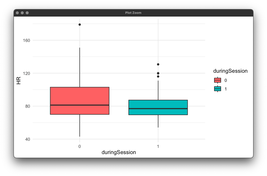
From here, I'll look at a boxplot comparing my heart rates both during and outside of a session:
# convert duringSession to factor
hr_mind[, duringSession := as.factor(duringSession)]

# look at boxplot
ggplot(hr_mind, aes(x = duringSession, y = HR, fill = duringSession)) +
  geom_boxplot() +
  theme_minimal()
This reminds me of a 2-sample t-test, let's remove the outliers and do that!
# remove outliers
hr_mind = hr_mind[,.SD[HR < quantile(HR, probs = 0.95)], by = duringSession]

# look at boxplot (again)
ggplot(hr_mind, aes(x = duringSession, y = HR, fill = duringSession)) +
  geom_boxplot() +
  theme_minimal()

# lm
mod = lm(HR ~ duringSession, data = hr_mind)
summary(mod)
> summary(mod)

Call:
lm(formula = HR ~ duringSession, data = hr_mind)

Residuals:
    Min      1Q  Median      3Q     Max
-41.911 -14.911  -3.911  11.743  43.089

Coefficients:
              Estimate Std. Error t value Pr(>|t|)
(Intercept)     84.911      0.476 178.377  < 2e-16 ***
duringSession   -7.654      1.183  -6.469 1.27e-10 ***
---
Signif. codes:  0 ‘***’ 0.001 ‘**’ 0.01 ‘*’ 0.05 ‘.’ 0.1 ‘ ’ 1

Residual standard error: 18.32 on 1765 degrees of freedom
Multiple R-squared:  0.02316,   Adjusted R-squared:  0.02261
F-statistic: 41.85 on 1 and 1765 DF,  p-value: 1.273e-10
Well there's statistical evidence to suggest that my heart rates during and outside mindfulness sessions is different, though practically it might be that great of a difference. It is, however, interesting that the variation in my heart rate is much smaller when practicing.
Example: Hiking Routes
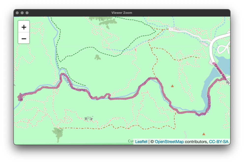
When exporting data, you'll also have a folder with gpx files that contain workout route information. I'm going to grab the file for my most recent hike and plot it:
# get hikes
hikes = workout_dat[workoutActivityType == "HKWorkoutActivityTypeHiking"]

# get most recent hike date
hike_date = as_date(hikes[endDate == max(endDate)]$endDate)

# fetch .gpx file
route_list = list.files("Data/apple_health_export/workout-routes/")
route = str_which(route_list, paste0(hike_date))
filename = paste0("Data/apple_health_export/workout-routes/",route_list[route])
hike_gpx = htmlTreeParse(file = filename, useInternalNodes = TRUE)

# get coords & elevation
coords = xpathSApply(hike_gpx, path = "//trkpt", fun = xmlAttrs)
elevation = xpathSApply(hike_gpx, path = "//trkpt/ele", fun = xmlValue)

# create data.table
hike_route = data.table(
  LAT = as.numeric(coords["lat",]),
  LON = as.numeric(coords["lon",]),
  ELEVATION = as.numeric(elevation)
)

# leaflet
leaflet() %>%
  addTiles() %>%
  addPolylines(data = hike_route,
               lat = ~ LAT,
               lng = ~ LON,
               color = "#AE2573")
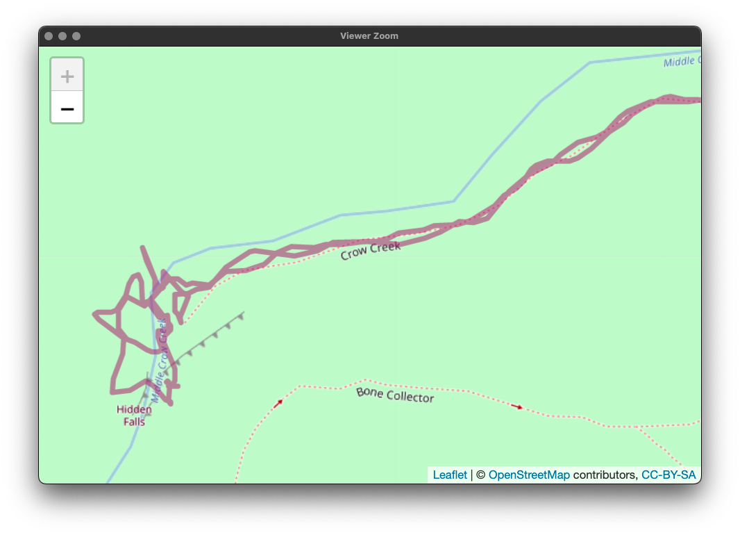
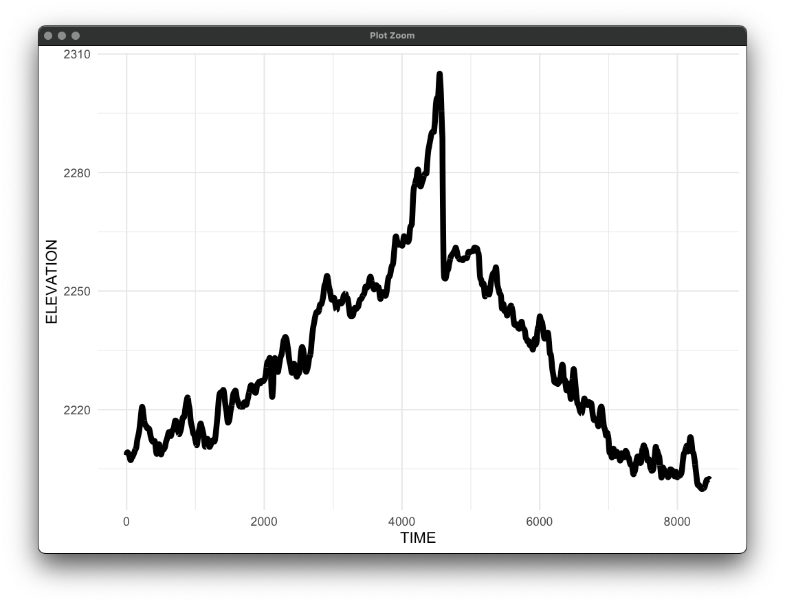
My most recent hike was to the Hidden Falls in Curt Gowdy State Park here in Wyoming. Let's see the plot: We can zoom in on the plot to see the level of detail the gpx files contain: Neat! We can also look at the elevation change during the hike:
# ggplot elevation
hike_route[, TIME := 1:.N]
ggplot(hike_route, aes(x = TIME, y = ELEVATION)) +
  geom_line(linewidth = 2) +
  theme_minimal()
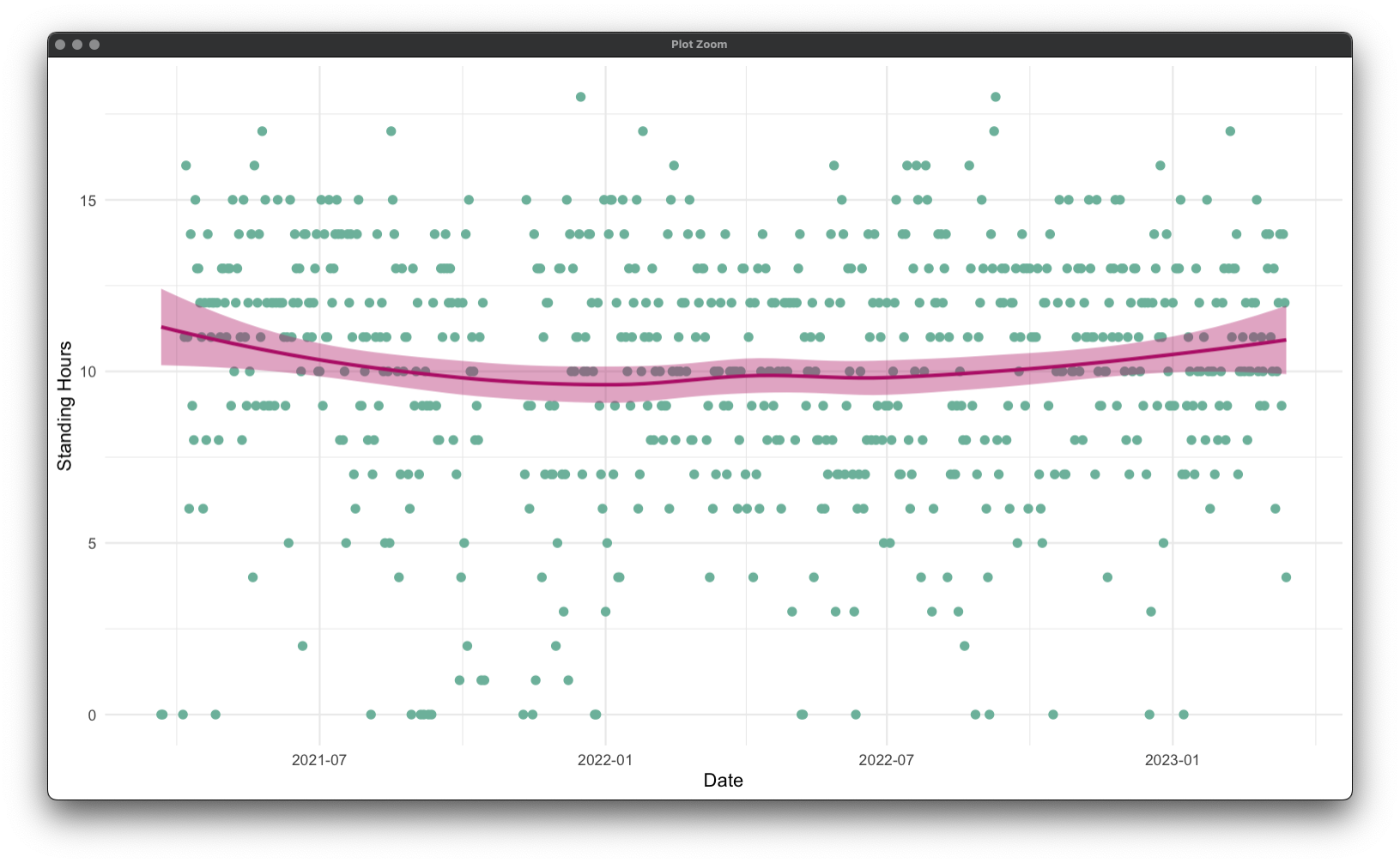
Example: Standing Hours
Finally, to work with the summary records, let's look at a plot of my standing hours over time. This time, no data manipulation is really required:
At any rate, there's a bunch of fun and interesting things to look at in the Apple Health data exports and this post has showcased a few of those things. I hope you have fun exploring!