A frequent problem in User Acquisition is to estimate ARPU (aka LTV when t->+inf) of the cohort — and a solid retention model is the foundation of any decent ARPU forecast.
A common approach to model retention is nonlinear asymptotic regression: y(t) = a + b/(c + t)
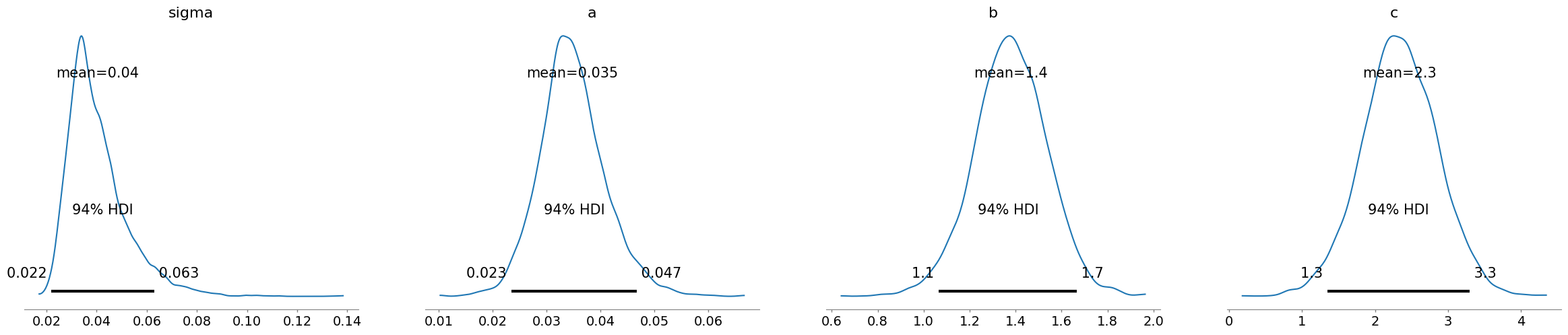
Think of it as: most users bail early, then things flatten out. Here, (a) is your long-term survivors (the loyal 2–3%), (b) is the big early drop, and (c) controls how fast the bleeding stops.
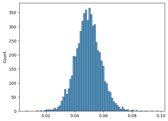
and there is how to implement a fully bayesian version of this model to properly deal with model uncertainty. As a bonus, it's possible to extend heteroskedasticity with cohort size.
"""
 uv tool run \
  --with pymc \
  --with arviz \
  --with numpy \
  --with matplotlib \
  --with seaborn \
  --with jupyter  \
  jupyter notebook --port=8888
"""

import pymc as pm
import arviz as az
import numpy as np
import matplotlib.pyplot as plt
import seaborn as sns

# time
x = np.array([1, 2, 3, 4, 5, 6, 7, 14, 28, 30, 60, 90 ])

# cohort retention
y = np.array([0.468, 0.339, 0.28, 0.245, 0.22, 0.202, 0.188, 0.131, 0.0908, 0.0847, 0.052, 0.0391])

with pm.Model() as model:
    sigma = pm.HalfNormal('sigma', 0.1)

    a = pm.HalfNormal('a', 0.1)
    b = pm.HalfNormal('b', 5)
    c = pm.HalfNormal('c', 1)
    # add heteroskedasticity as error in tail should be smaller than in head
    # just make sure it doesn't explode at t=0
    # ln(0+1) + 1 = 1
    # ln(100 + 1) + 1 = 5.61
    y_sigma = sigma / (np.log(x + 1) + 1)
    mu = a + b/(x + c)
    y = pm.Normal('y', mu=mu, sigma= y_sigma, observed=y)

    idata = pm.sample(1000, target_accept=0.95)
    ppc = pm.sample_posterior_predictive(idata, model=model)

az.plot_posterior(idata)
X = ppc.posterior_predictive.y.stack(z=('chain', 'draw')).to_numpy() # (T, draw)
def plot():
    for i in range(0,500):
        plt.plot(x, X[:, i], color='g')
    plt.plot(x, y,'x', color='b')
    plt.show()
plot()
# uncertainty on 90th day prediction
sns.histplot(X[-1, :])