Bayesian Switch-Point Detection: Catch the Exact Day Metrics Changed

A common problem when running User Acquisition at scale (or any marketing activity) is detecting if performance is changing over time - and more importantly, exactly when.

The usual manual way: export daily data from your BI tool (Meta Ads, Google Ads, AppsFlyer, etc.), paste it into Excel, and squint at the charts until something looks off. Works for a week, fails at scale.

Here’s a better way: a Bayesian change-point detection model that assumes two regimes (‘before’ and ‘after’) and finds the most probable switch day - automatically, with uncertainty quantified.

import pandas as pd
import pymc as pm
import arviz as az
import seaborn as sns


# time_1d, impressions, p, ctr, arpu
df = pd.read_csv('data.in.csv').sort_values(by='time_1d').reset_index().assign(
  idx=lambda x: x.index # convert dates into numbers, first day is 0 etc
)

with pm.Model(coords={'t': {'before': 0, 'after': 1}}) as model:
    impressions = pm.Normal("impressions", 
                            mu=200_000,
                            sigma=70_000,
                            dims='t')
    
    sigma_p = pm.HalfNormal('sigma_p', 0.005)
    sigma_ctr = pm.HalfNormal('sigma_ctr', .05)
    sigma_arpu = pm.HalfNormal('sigma_arpu', 0.1)
    
    p = pm.Beta('p', mu=0.01, sigma=sigma_p, dims='t')
    ctr = pm.Beta('ctr', mu=0.1, sigma=sigma_ctr, dims='t')
    arpu = pm.Gamma('arpu', mu=0.15, sigma=sigma_arpu, dims='t')

    # switchpoint
    tau = pm.DiscreteUniform('tau', lower=0, upper=df.idx.max())
    
    idx = pm.math.switch(df.idx.values < tau, 0 , 1)
    
    pm.Poisson('y_impressions', mu=impressions[idx], observed=df.impressions.values)
    pm.Beta('y_p', mu=p[idx], observed=df.p.values, sigma=sigma_p)
    pm.Beta('y_ctr', mu=ctr[idx], observed=df.ctr.values, sigma=sigma_ctr)
    pm.Gamma('y_arpu', mu=arpu[idx], observed=df.arpu.values, sigma=sigma_arpu)

    # run only once chain to avoid label switching
    idata = pm.sample(5000, chains=1, target_accept=0.95)

az.plot_posterior(idata.posterior, var_names=["impressions", "tau"])

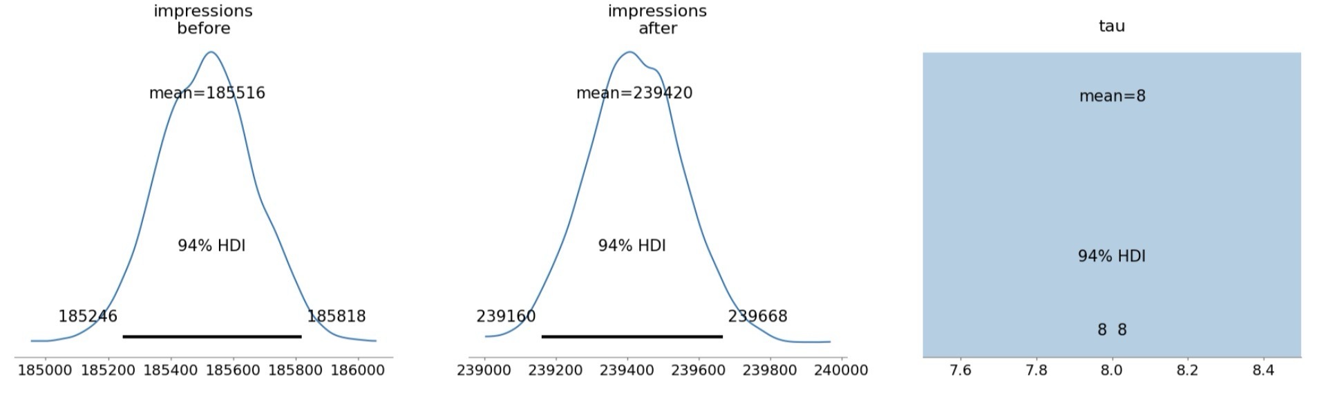
In my case, the model detected a razor-sharp switch point on day 8 with 99.9% posterior probability. Impressions jumped from a pre-switch mean of 185,516 (94% HDI [185,246 – 185,818]) to a post-switch mean of 239,420 (94% HDI [239,160 – 239,668]) — a statistically significant +29% surge in volume, with zero overlap between the two posterior distributions.

One of the best parts of the Bayesian approach: when the data is truly ambiguous, the model doesn’t force a fake “single day” answer. Instead, the posterior for τ (the switch point) stays flat across an interval, honestly telling you “any day in this window is equally likely.” No false precision, no pretending the switch was on day 12 when the evidence supports days 10–15 just as much.

Inspired by Chapter 1 of Bayesian Methods for Hackers