I often get asked about what steps I follow when we kickoff a new coding project. It’s important to mention that I’m part of a team of geospatial programmers so we do things slightly differently to web developers and data scientists. We don’t do scrums, sprints and all the other shenanigans, and we rarely do feature branches on git. Yes some steps have been inspired from industry standards but have been simplified for our team’s needs. We have a different approach that’s fit for purpose and it works. So without a further ado let’s dive into it.

As geospatial professionals we usually have to handle and process large volumes of spatial data. These are either saved on our postgres server or on a dedicated remote machine (that’s shared between my team members). For the purposes of today's exercise, let’s call the latter the N drive.

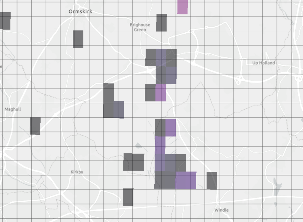
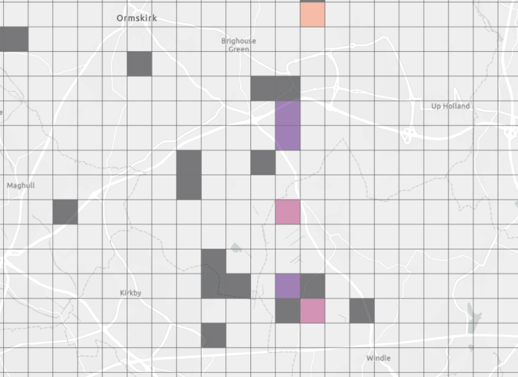
What I have been tasked to do today, pardon me if you’re unfamiliar with the GIS lingo, is to convert a number of geotiffs showing a timeseries of fire distributions in the UK to a new grid system (the 1x1km one we use to publish our emissions maps). The following maps present the before and after.

Initialising and setting up the repository 🚀

So how do we do that? We code and we code a lot, so it's best practice to use a version control system for our work. But contrary to navigating to a local path and following the git init and the rest of the commands, I prefer to find the desired location on gitlab and create the repo with a README file. We use gitlab in the company for our version control which has the same functionality as github, if you're more familiar with it. I prefer gitlab's site for my git init as its UI is simple and easy to navigate and it, simply, just works. So after that, I clone the project on my local D drive and run the following commands.

git clone git@companys-path-hidden/wildfires.git
git cd wildfires # to navigate to the local path of the repo
git status # ensure that I'm working in a git repo
git checkout -b develop main # create the develop
git checkout -b naei22-ce develop # create my working branch

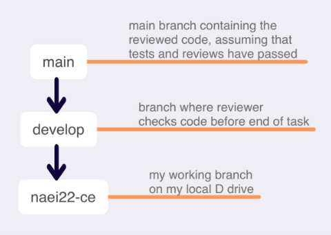
As I mentioned previously, we don't do feature branches but we follow the following schematic. The allows us the team to work on multiple branches and push to the develop branch our various updates. But for today lets assume that I will undertake this task on my own. FYI my branch has been named like this under this convention: project_name (naei), year (22) and initials (ce). The year has been set to 2022 as we always compile our emissions inventory in two years in arrears.

Following, the 'checkout' of our branch, I run the following commands for the gitignore file.

touch .gitignore
notepad .gitignore

This opens a notepad where the following paths are inserted in the following syntax so they aren't 'ignored'. Essentially I'm ignoring everything (through /*), except the paths below.

# Folders to ignore
/*
!/README.md
!/jupyter/
!/images/
!/docs
!/.gitignore
jupyter/.ipynb_checkpoints

I then, using VS code, choose all available files to commit and push to remote. The sole reason I use VS code here and when pushing to remote is to visualise the git graph - I can check each branch, its status and progress against each other in a simple and intuitive way. Okay, these steps have so far been the preparatory ones, so let's get ready for the bread and butter of geospatial programming and start writing our code.

Programming 👨🏼‍💻

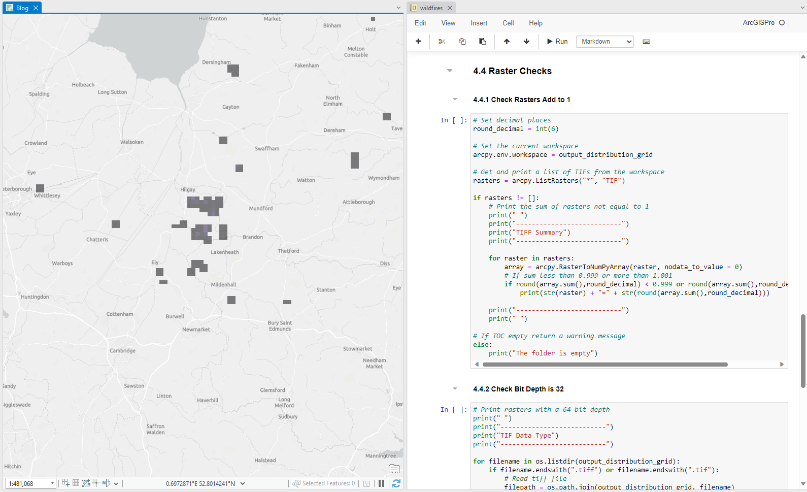
As geospatial programmers we tend to write our code in python (in addition to R and SQL). Python, in my opinion, processes spatial data more efficiently hence why I preferred this language for this exercise. I'm also using ArcPy (a flavour of Python developed by ESRI). This enables me to have a split screen of the notebook, in ArcGIS Pro, and visualise the map that gets updated after each run of a 'code chunk' (see a bonus screenshot at the end of this entry). So now I create the main notebook for this exercise in the 'jupyter' folder. Unfortunately, I can't share the exact code but the sections below provide the breakdown of the steps followed along with some pseudocode.

The first thing the precedes the setup is to write a brief description of what the task entails so it can be understood by another technical person (usually by another team member). This is different to the contents of the main README which provides details to someone who hasn't and won't work directly on the notebooks and functions (.py files) of the project. The description of this notebook is as follows:

Description: The Wildfires' distribution grids used in the NAEI are based on an aggregation of 3 Land Cover classes (arable, vegetation, forest) and therefore do not reflect the location and duration of fires that have taken place in the UK. This notebook utilises data provided by Aaron Davitt (Climate TRACE) to create new distribution grids.

The 4 main steps are:Setup
Polygonise rasters
Intersect Climate TRACE Grids with NAEI Grids
Join Emissions to Gridcodes and Export Normalised Distribution Grids

Original Author: Christopher Evangelides
Date: January 2023 (NAEI 2021)

Maintainer: Sian Hows
Date: December 2023 (NAEI 2022 update)

Modified by: Sian Hows
Date: Decemeber 2023

Setup

The following libraries are the ones used by the team and are set as the defaults in new python notebooks

# Load libraries
import os
import arcpy
import numpy as np
from arcpy import env
from arcgis.features import GeoAccessor, GeoSeriesAccessor
from arcgis import GIS
import pandas as pd
from pandas import Series, DataFrame
import requests
import zipfile
import shutil

The setup also contains the parameters and relevant paths of interest for the project. In the abridged parameters below, I wanted to highlight that the ROOT folder and subsequent paths are set to the N drive, where as I mentioned before, it stores, and now, reads the large volumes of spatial data. This means that when we collaborate as a team, each of us works on our local D drive (for the repo and coding) but we point to the same N drive to read and write spatial files.

inventory_year = 2022
naei_year = str(inventory_year)

# Define ROOT and folders of interest
ROOT = r"N:\naei" + naei_year[2:4] + "\9_mapping\Wildfires" 
...

I wish I could share the exact code, but for now I can only share the steps followed to get our grids (geotiffs) of interest.

1 Setup1.1 Libraries
1.2 Parameters
1.3 Functions # load functions from the .py files
1.4 Save raw files # via an API to the N drive
2 Polygonise rasters2.1 Convert Raster to BNG UK Points Layer
2.2 Create a Fishnet
2.3 Combine Point Layers with the fishnet
3 Intersect Climate TRACE Grids with NAEI Grids
4 Join Emissions to Gridcodes and Export Normalised Distribution Grids4.1 Forest Layers
4.2 Shrub and Wetland Layers
4.3 Create Tifs from Rasters
4.4 Raster Checks

I guess I can share 4.4 and a code chunk of our checks. This one checks that each exported raster (geotiff) adds up to 1. This is particularly important to ensure that emission totals (compiled in a different exercise by our non-GIS colleagues) are presented and distributed accurately across the UK.

# Set decimal places
round_decimal = int(6)

# Set the current workspace
arcpy.env.workspace = output_distribution_grid

# Get and print a list of TIFs from the workspace
rasters = arcpy.ListRasters("*", "TIF")

if rasters != []:
    # Print the sum of rasters not equal to 1
    print(" ")
    print("---------------------------")
    print("TIFF Summary")
    print("---------------------------")

    for raster in rasters:
        array = arcpy.RasterToNumPyArray(raster, nodata_to_value = 0)
        # If sum less than 0.999 or more than 1.001
        if round(array.sum(),round_decimal) < 0.999 or round(array.sum(),round_decimal) > 1.001:
            print(str(raster) + "=" + str(round(array.sum(),round_decimal)))

    print("---------------------------")
    print(" ")

# If TOC empty return a warning message
else:
    print("The folder is empty")

That's it for today. I hope you enjoyed the steps we follow in the team when working and manipulating spatial data. Ohh, yes here's the bonus screenshot of the beautiful setup after running the check code chunks. Let me know what you think.

Behind the scenes of geospatial coding 👾

Initialising and setting up the repository 🚀

Programming 👨🏼‍💻

Setup