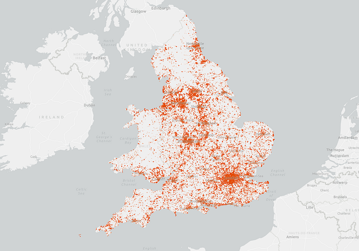
That most certainly is not linked to my ability to code but more on the freedom I had as a student. What I mean is that I recently worked during the Good Friday and Easter Monday bank holidays and it was certainly liberating and got me to reminisce my days as a student - specifically not having to follow the 9-to-5 schedule and being bombarded with emails, IMs and meeting reminders. It coincided with a nice piece of work I had to do for one of our clients - using interpolatory methods to estimate the price of square footage for each industrial building across Great Britain where data haven't been gathered. And today I’d like to share these chunks of code along with some maps that were created along the way (confidentiality is preserved throughout).
For this exercise I used ESRI’s ArcPy environment 🐍 (unfortunately I can't publish the git repo).
Let’s start by importing our libraries and making sure that the ArcPy environment has been loaded correctly
For this exercise I used ESRI’s ArcPy environment 🐍 (unfortunately I can't publish the git repo).
Let’s start by importing our libraries and making sure that the ArcPy environment has been loaded correctly
%%capture
from arcgis.gis import GIS
from IPython.display import display
mygis = GIS("pro") # Use ArcGIS Pro to connect
myaccount = mygis.users.me

import numpy as np
import os
import numpy as np
import pandas as pd
import csv
import arcpy
from arcpy import env
from arcpy.sa import *
Set paths and parameters
# Boooyakasha esketiiit
ROOT     = r"Q:\Delivery\GISdata\project_root" # renamed folder to preserve confidentiality
gdb_name = r"main.gdb"
gdb_path = os.path.join(ROOT, "arcpro", gdb_name)

# Raw table with partly filled records on price of industrial sites
interpolation_path = os.path.join(ROOT, "interpolation")
raw_data           = os.path.join(interpolation_path, "estimating_floor_area.csv")
symbology_pre      = os.path.join(interpolation_path, "point_data.lyrx")
raster_post        = os.path.join(interpolation_path, "out_raster.lyrx")

# Raw point data - point layer (geom)
point_data         = r"point_data"
point_data_path    = os.path.join(gdb_path, point_data)

# define location of interpolated prices - raster
interp_raster      = r"natural_interp_raster_0_0001"
interp_raster_path = os.path.join(gdb_path,interp_raster)

# define location of Extract Values to Points
interp_points      = r"interp_points"
interp_points_path = os.path.join(gdb_path, interp_points)
Convert raw table to Points (geom)
arcpy.management.XYTableToPoint(raw_data,
                                point_data_path,
                                "longitude",
                                "latitude",
                                None,
'GEOGCS["GCS_WGS_1984",DATUM["D_WGS_1984",SPHEROID["WGS_1984",6378137.0,298.257223563]],PRIMEM["Greenwich",0.0],UNIT["Degree",0.0174532925199433]];-400 -400 1000000000;-100000 10000;-100000 10000;8.98315284119521E-09;0.001;0.001;IsHighPrecision')
Apply Symbology
arcpy.management.ApplySymbologyFromLayer(point_data,
                                         symbology_pre,
                                         None,
                                         "MAINTAIN")
Add Spatial Index
arcpy.management.AddSpatialIndex(point_data, 0, 0, 0)
Run Natural Neighbor Interpolation
# Create new column called "price_x_meter_2"
arcpy.env.addOutputsToMap = 0
print("Creating new field")
arcpy.management.CalculateField("point_data",
                                "price_x_meter_2",
                                "!price_x_meter!",
                                "PYTHON3",
                                '',
                                "FLOAT",
                                "NO_ENFORCE_DOMAINS")

print("Creating the interpolated raster")

# Process takes quite some time at GB-level, approx 1hour
out_raster = arcpy.sa.NaturalNeighbor(point_data,
                         "price_x_meter_2",
                         0.0001); out_raster.save(interp_raster_path)
# 0.0001 refers to the size of the raster cell which in this case is 0.0001 m. It was  chosen to provide more accurate and reliable results within in a sensible timeframe (approx. 1 hour).

print("DONZOW")
Apply Symbology
arcpy.management.ApplySymbologyFromLayer(interp_raster_path,
                                         raster_post,
                                         None,
                                         "MAINTAIN")
Extract Values to Point
arcpy.sa.ExtractValuesToPoints(point_data,
                               interp_raster_path,
                               interp_points_path,
                               "NONE",
                               "ALL")
Apply Symbology
arcpy.env.addOutputsToMap = 1
arcpy.management.ApplySymbologyFromLayer(interp_points_path,
                                         symbology_pre,
                                         None,
                                         "MAINTAIN")
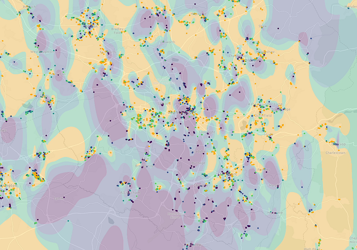
We can see here the interpolated values (class values are hidden for confidentiality) overlayed on the raster (smooth surface; coloured background). Class breakdowns are consistent between the two layers for a visual comparison - the results, at least from this map, look promising (scatter plot below provides more insights).
Rename RASTERVALU field
arcpy.management.AlterField(interp_points_path,
                            "RASTERVALU",
                            "raster_x_meter_interp",
                            "raster_x_meter_interp",
                            "FLOAT", 4,
                            "NULLABLE",
                            "DO_NOT_CLEAR")
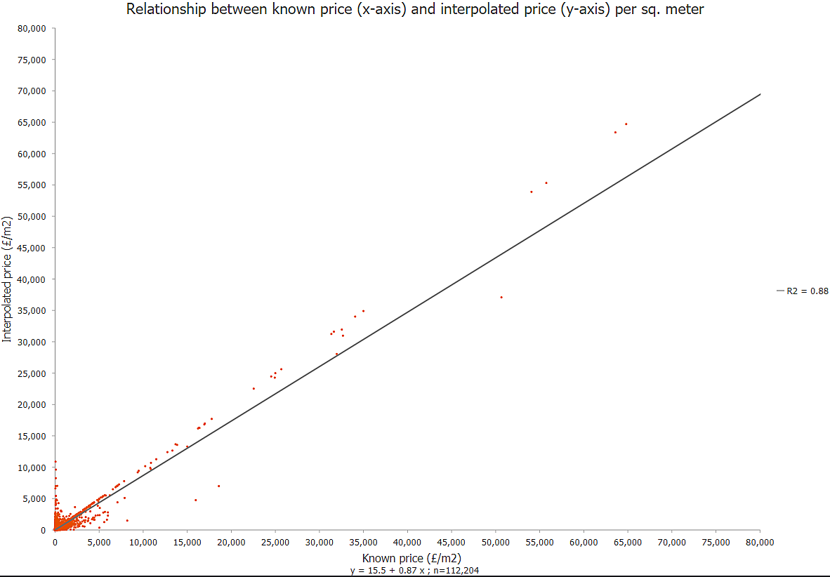
…and now let’s do a simple comparison to the points (i.e. industrial sites) that we used for the interpolation (known values - our independent variable).

notta bad R2 value right? (in the most Italian accent)

Export table (postgres-ready)
Prepare csv that is ready for further analysis on postgres
arcpy.conversion.TableToTable(interp_points_path,
                              interpolation_path,
                              "method1_interpolation.csv",
                              '',
                              '', # fields hidden for confidentiality
                              '')
