Spatial Clustering: Love Letters (Part 1: Data Cleaning & Setup)
Handwritten Greeting Cards
In my introductory blog post, I mentioned that Her is one of my favorite movies. I was once told that it "makes sense" why it's up there for me. Years later, I still have no idea if that's a good thing or not - I guess I'll leave that one up to you. Regardless, let's ruin the movie by overthinking a toy example, shall we?
One of the bits that I find endearing is that Theodore, our protagonist, works for a company called Handwritten Greeting Cards where he (see if you can follow) writes greeting cards. He writes these letters from other people to their chosen recipient which is amusing to me because (a) in my mind, the whole point of sending a personal letter is to have written it yourself and (b) this seems like a totally plausible company to exist in our modern world. Not to mention that he doesn't hand-write the cards to begin with!
Now the question I'm sure you're asking is: "Garrett, what does this have to do with ambulances?" What a great question (and very natural one I might add)!
I'm currently working on a project trying to optimize ambulance placements in Wyoming on the county level. The question is, in essence, given X number of ambulances, where should they be placed within each county to minimize response time? Because that project involves sensitive information, my goal here is to demonstrate the methodology and findings from that project in a properly absurd and fictional way. For good measure, or for good fun, you should probably throw on Arcade Fire's score for the movie while you're here!
The Problem
Our scenario will provide the same services as Handwritten Greeting Cards but with a bit of rebranding. Due to ever-shortening attention spans and a need for instant gratification approaching the speed of light, our company has ditched the name Handwritten Greeting Cards in favor of Handwritten Greeting Cards (Now!).
What we want to take on is the delivery phase of the operation and make that speedier. So, a customer requests a card, we write it, and send it electronically to something like those Amazon delivery vans you might see out and about - we'll be printing our greeting cards inside of our vans. Once a greeting card is printed inside the van, we'll deliver it straight to the recipient's address.
What we want to know is, given a certain town/city/county, how many vans should there be and where should we place these vans in order to minimize the time between our writers finishing a card and the time it is delivered.
Following Along
From here on out, I'll be referencing data and scripts with in my Love Letters Github. Fork and desecrate, this is the way.
Data: Download & Setup
Because I'm familiar enough to know better, one of the first places we're looking to launch our service in is Casper, Wyoming. For the sake of this example, I'll assume that the amount of cards delivered to a specific place is a function of population and time of year.
The United States Census Bureau's 2020 Decennial P.L. 94-171 Redistricting Census Data has population counts per census block as well as some demographic information, though sadly no age data is available from the 2020 census as of yet. We'll need a few things from that page:
The wy2020.pl.zip file which can be found in the Legacy Format Summary Files.
Once you've unzipped the wy2020.pl files where you can reach them (I put them in cens_files folder within my R project directory), you can just run the pl_all_4_2020_dar.r script in the import scripts, changing the pl file locations to where you've put them. Or, easier, just use my edited version: 1-prolog_import.r if you're following using my Github repo. The only other thing I changed is saving the combined data as an rds file.
saveRDS(combine, "R_Objects/cens_import.rds")
Data: Cleaning
Now we can go ahead and clean the data (2-data_setup.r). We can read in the combined data as a data table (my preferred format) and select the columns we're interested in since there's 400 of them. For this example, all we'll need is GEOCODE (so we can filter down to individual census blocks), POP100 (population count), latitude, longitude, and PLACE (so we can merge in place names and filter down to the Casper area).
For some reason, latitude is coded with a "+" at the beginning of each when read in. We can use gsub() to get rid of that. We also want to make sure we're only getting census block information (as opposed to state-level, county-level, town-level summaries), so we'll subset to observations where GEOCODE is exactly 15 characters long. Finally, we'll set the key to be the PLACE column so we can merge this data and our Name Lookup Table:
library(data.table)
library(stringr)

cens = as.data.table(readRDS("R_Objects/cens_import.rds"))
cens = cens[, .(GEOCODE, POP100, INTPTLAT, INTPTLON, PLACE)]
cens[, INTPTLAT := gsub("\\+", "", INTPTLAT)] # get rid of "+" in latitude coordinates
cens = cens[str_length(GEOCODE) == 15] # filter to just census blocks
setkey(cens, PLACE)
Make sure the NAMES_ST56_WY.zip is unzipped somewhere you can grab it. I unzipped mine in R Project Directory > cens_files > names. We can use data.table::fread() to read both the CDP and city .txt files. We'll rbind them together (since their place codes are unique) and remove more columns we don't need. We'll also set the key to be the place code so we can merge the names back into our original data. Finally, we'll go ahead merge the two and remove observations where there is no city or CDP associated:
# import names
CDP_names = fread("cens_files/names/NAMES_ST56_WY_CDP.txt")
CITY_names = fread("cens_files/names/NAMES_ST56_WY_INCPLACE.txt")
names = rbind(CDP_names, CITY_names) # combine
names[, c("STATEFP", "NAMELSAD") := NULL] # remove more detailed name & state code
names[, PLACEFP := as.character(PLACEFP)]
setkey(names, PLACEFP)

# merge
cens = cens[names]
cens = cens[!(is.na(NAME))]
Finally, let's narrow our dataset down to the Casper area. Here I'm including the names of Casper and its extensions, only keeping census blocks that are populated, and doing some more general cleaning.
# filter to Casper Area
cens = cens[NAME %in% c("Casper", "Mills", "Evansville", "Casper Mountain")]
cens = cens[POP100 != 0]
cens[, ID := 1:.N] # create ID variable (to replace GEOCODE)
cens[, c("NAME", "PLACE", "GEOCODE") := NULL] # remove unused cols after reduction
setnames(cens, c("Population", "Lat", "Lon", "ID")) # clean colnames
setcolorder(cens, "ID") # ID first
cens[, Population := as.numeric(Population)][, Lon := as.numeric(Lon)][, Lat := as.numeric(Lat)]
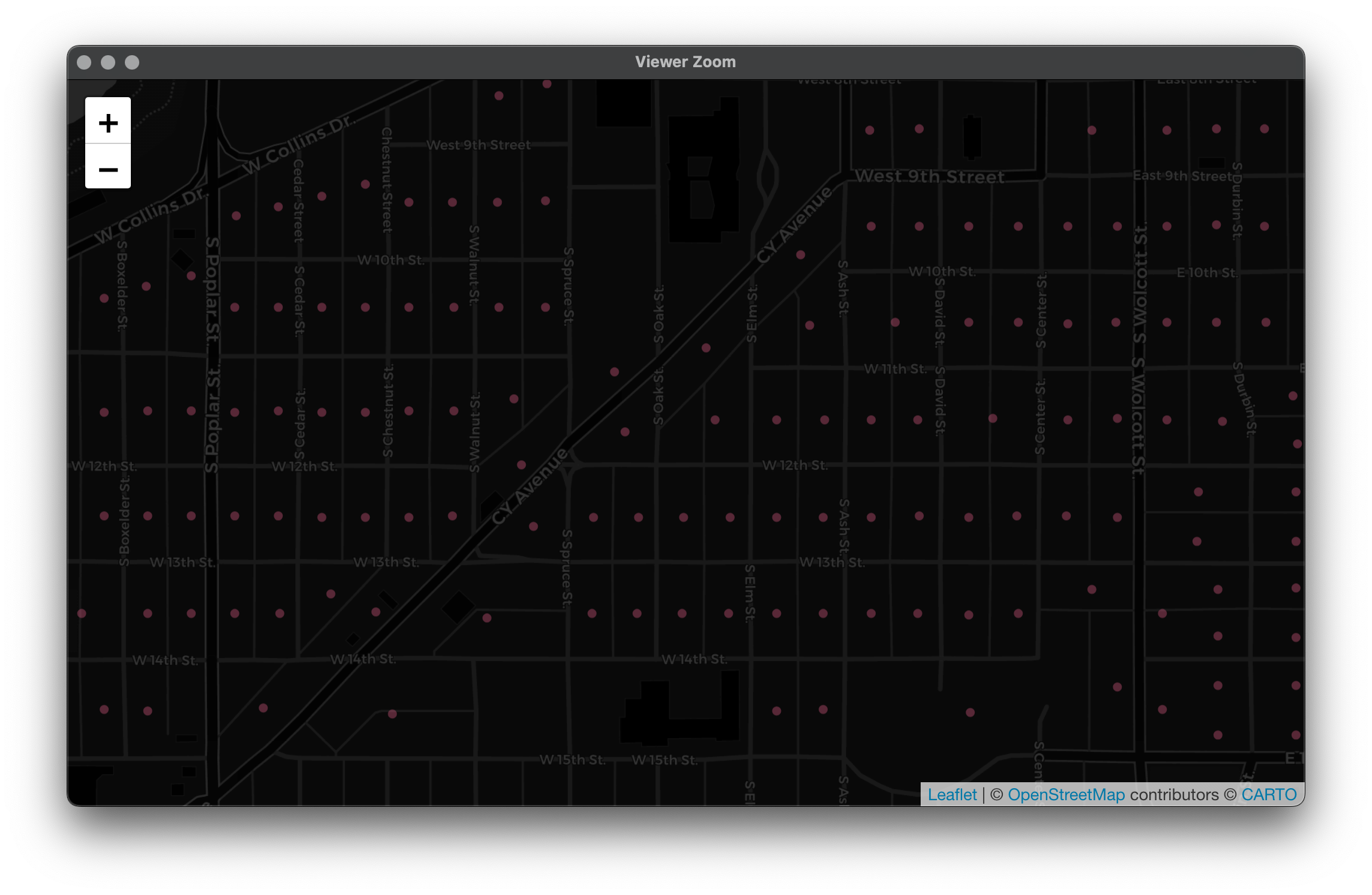
If we zoom in, we can finally see what a census block is. Remember for each one of these blocks we have a population count:
Generating Letter Deliveries
Recall that we're assuming the number of letters to a given census block is a function of population and time of year. To generate a predicted number of letters per census block, we'll need to expand our data to include months of the year. We can then use the month number in tandem with the population to make up a variable rate parameter (by month) and generate predicted numbers of letters from a Poisson distribution using rpois().
Here I'm saying that for the months of November, December, and January, cards are generated at twice the rate they normally would be. For February, it'll be 3 times that (what with Valentine's Day and all). Our check looks good:
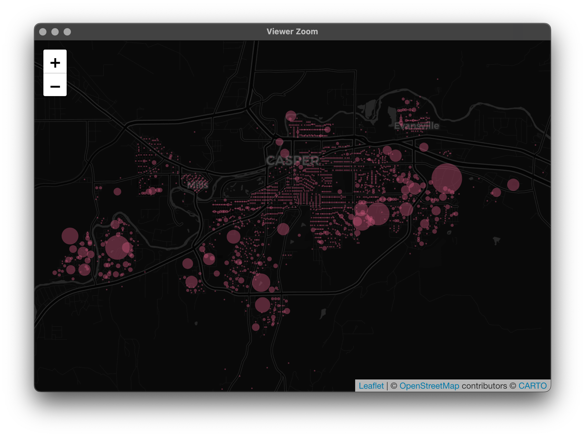
Finally, let's make another map to look at the average number of letters per census block using variable radius sizes where the larger the circle, the more cards delivered:
# map average calls
cens = cbind(cens, monthly[, mean(Response), by =  ID]$V1)
setnames(cens, "V2", "Avg_Call")

leaflet(cens) %>%
  addProviderTiles(providers$CartoDB.DarkMatter) %>%
  addCircleMarkers(~Avg_Call, lng = ~Lon, lat = ~Lat,
                   stroke = F, fillOpacity = .4,
                   color = "#d0587e")
Most of the blocks with high predicted calls are blocks with larger apartment complexes and the like, so this looks good to me!
# save
saveRDS(monthly, "R_Objects/monthly.rds")
saveRDS(cens, "R_Objects/cens_cleaned.rds")
What's Next
We now have everything we need to go ahead and get started on answering our questions:
How many vans should we allocate for the Casper area?
Where should we place the vans?
To get at these, we'll explore using spatial clustering algorithms with some interesting twists. Ominous, no? As a taster, we'll be using OSRM to obtain a distance matrix of real drive times for these census blocks.