Spatial Clustering: Love Letters (Part 3: Equalify)
Project Recap:
In Part 1, I motivated this spatial clustering scenario as an optimization problem based on the movie Her. As the executives of Handwritten Greeting Cards (the company the protagonist works for), we are proposing a new delivery method wherein cards are sent electronically to vans in which they are printed and delivered to the recipient. In essence, we're ditching traditional delivery means in favor of a Uber/Lyft style approach to reduce the time between a card being written and it being received as much as possible.
Using 2020 Decennial Redistricting data, we were able to narrow our scope down to census blocks in the Casper, Wyoming area and fabricate estimates for the number of cards each block would receive based on population count and time of year (higher volumes are expected around holidays, etc.).
What we really want to know is the following:
How many vans should we allocate for Casper, WY?
Where should these vans be placed?
In Part 2, we set up a local Open Source Routing Machine (OSRM) server and were able to obtain a distance matrix of travel times instead of one based on Euclidean distances. Our hope was that shifting distances into a more realistic space would yield more realistic clustering results. Using the WeightedCluster package, we used the PAMonce algorithm on both travel time and Euclidean distance matrices, using the estimated number of calls per census block as the weights for that block. We generalized code and found solutions for 2-10 vans for both distance matrices. We wrote more in-depth leaflet code and compared solutions. Our takeaways were as follows:
Using the travel time distance matrix generally yielded a reduction in average travel time within each cluster. When compared with solutions utilizing Euclidean distances, we found that travel time solutions were more efficient from a time standpoint.
We observed one solution that effectively balanced the workload between the vans - each van would deliver a similar number of letters. This was an intriguing result and it was hypothesized that finding a clustering solution balancing workloads between vans that also utilized travel time might be optimal.
Unfortunately, as discussed, I could find no such algorithm during my search of the web. So, I decided to try my hand at writing my own.
Balancing the Force - Equalify:
In hindsight, what this algorithm does isn't anything all that special. That being said, it did take quite a bit of thinking through to reach a working function. It isn't efficient in the slightest (due to for loops) but it yields some interesting results. Grab the 5 - equalify.R script from the love_letters GitHub Repo and let's dive in!
The usual here with the addition of the pushoverr package. A few posts back, I argued that BrowseURL() can be used to signal the end of code running better than beepr::beep(). pushoverr takes this concept and extends it further by allowing you to send a push notification to any of your devices. Its use case and scope is a little larger than what this project necessitates, but I thought it might be a cool bonus code-wise. It's entirely optional here. Feel free to jump to "The Algorithm" header if you don't want to bother with it.
pushoverr Configuration:
Download the Pushover app from the Google Play Store or from Apple's App Store. You'll be prompted to create an account and after you do so, you'll be given a 30 character long user key. Halfway done!
Next, navigate to the Pushover application builder (you'll have to sign in first). Give your app a name and accept the ToS, everything else is optional. I used "R" as my application name and gave it an RStudio icon. Back on your Pushover dashboard, navigate to your app and a 30 character API key will show up. You're all set from here!
And, with some luck your phone will do phone-y things:
The Algorithm:
Getting to the thing itself, we'll need to import our data, previous clustering results, the travel time matrix, and our distance matrix. Setting up some debugging code here for our function too:
The only new ideas are a threshold variable and a couple of iteration controllers. In the same way as we built our function that utilizes the wcKMedoids function, our function will essentially output a data.table with summaries and cluster assignments. We'll start by copy the census data as to not modify the original:
  # copy data
  data = copy(census_data)
  setkey(data, ID)
Now for more of the thinking bits. We want to restrict our vans to being placed in/around high utilization areas. Using the threshold set in our function, only census blocks where the number of letters is above the Xth percentile (if unchanged, the default would be the 90th percentile). By reducing the number of places our vans can be placed in this manner, we should only be placing vans where we expect high utilization. We'll then calculate a goal - the ideal number of letters delivered to each cluster. This is simply the total number of letters divided by the number of vans we want. Finally, some custom which.min functions that will make playing with our travel time matrix easier.
  # select candidates
  cand = data[Avg_Call >= quantile(data$Avg_Call, threshold)]
  cand = as.character(cand$ID)

  # goal population per van
  goal = sum(data$Avg_Call)/n_vans

  # custom min functions used
  which.min.name = function(x) {
    which = which.min(x)
    names(which)
  }
  which.pmin = function(...) {
    apply(cbind(...), 1, which.min.name)
  }
With our debugging settings, our goal number of letters delivered per van is
> goal
[1] 624.9722
What we'll do from here is randomly sample from the candidate blocks for starting locations. After writing one of the initial versions of this algorithm, I noticed these starting blocks/locations heavily affect the outcome so the iters variable in the function controls how many times to start the algorithm in different places. After getting the results from each run from 1:iters, we can pick a "best" solution based on evaluation criteria.
# overall loop (this eases starting bias concerns)
  results = data.table()
  for (iter in 1:iters) {
From there, the actual algorithm is pretty simple. We can start by sampling from our list of candidate blocks. Once selected, we can pick out these columns from our travel time matrix.
While testing, I noticed that very rarely, the candidates wouldn't select itself as the closest if the distance from it to another candidate is 0. This happens very rarely but can happen, so this fixes that.
Now the setup is complete! From here, we'll loop until a solution is found or until the subiters argument demands we break the loop. First, we'll check if any of our candidates has met our goal, giving some leeway here as landing exactly on our ideal is virtually impossible.
# reallocation process
satisfy = F
it = 1
assign_table = data.table()
while (satisfy != T) {
# how far from goal
goal_eval = time_subset[, .(Avg_Call = sum(Avg_Call)), by = Clust]
goal_eval[, Off := Avg_Call - goal]
goal_eval[, COMP := fifelse(abs(Off) <= goal*(1-threshold), 1, 0)]
In this case, block 1344 met our criteria to be marked as completed. We'll have to check it off now. Below, the done variable notes the ID (1344) and id_done saves all of the census blocks assigned to 1344. Then there's some logic on what to do from there. We'll save the assignments to a table, break the while loop if a solution has been reached, and remove 1344 and any of the blocks that were assigned to it from our valid candidates.
# reduce possible
done = goal_eval[COMP == 1]$Clust
id_done = time_subset[(Clust %in% done)]$ID
# save completed
if (length(done) >= 1) {
assign_table = rbind(
assign_table,
time_subset[ID %in% id_done, .(ID, Clust, min_time)]
)
# if completed stop
if (length(unique(assign_table$Clust)) == n_vans) {
satisfy = T
break
}
# remove completed ID's from valid candidates
valid = valid[!(valid %in% assign_table$ID)]
}
Before, we had 205 valid candidates:
> length(valid)
[1] 205
After the above is run, we only have 158:
> length(valid)
[1] 158
From there, we just need to re-sample, rinse, and repeat, breaking if the iteration maximum has been reached or if each cluster is within the threshold of the goal.
# re-sample from candidate list
selected = sample(valid,
n_vans - length(unique(assign_table$Clust)),
replace = F)
selected = c(selected, "ID")
# find travel times from time matrix
time_subset = time_mat[, ..selected]
time_subset[, Avg_Call := data$Avg_Call]
# make sure ID's done aren't re-assigned
time_subset = time_subset[!(ID %in% assign_table$ID)]
    # find which selected minimizes travel time
    time_subset[, min_time := do.call(pmin, .SD),
                .SDcols = selected[selected != "ID"]]
    time_subset[, Clust := do.call(which.pmin, .SD),
                .SDcols = selected[selected != "ID"]]
    # fringe case - ensure selected select themselves
    time_subset[ID %in% selected, Clust := ID]
# break while loop if it can't find solution
it = it +1
if (it == subiters) {
assign_table = rbind(assign_table,
time_subset[, .(ID, Clust, min_time)])
break
}
}
After the while loop has processed, we need to create the evaluation criteria and normalize cluster numbers.
After this piece runs, we'll have iters (50) clustering solutions to choose from. We'll pick the one that minimizes our critera (some extra logic in case more than 1 solution minimizes it). Finally, just like last time, we'll create a Medoid column, get assigned travel times, get the average travel time per cluster, and the population per cluster.
  # pick which iteration 1:iters did best
  minOV_EVAL = min(results$crit)
  results = results[crit == minOV_EVAL]

  # if more than 1 optimal, sample
  if (nrow(results) != nrow(data)) {
    it_samp = sample(results$it, 1, replace = F)
    results = results[it == it_samp]
  }

  # stamp placements, bind to original data
  results[, Medoid := fifelse(ID == Clust, 1, 0)]
  results = results[, .(ID, Clust = clust, Medoid, Clust_ID = Clust)]
  setkey(results, ID)
  setkey(data, ID)
  data = data[results]
  setkey(data, ID)

  # get travel times to from assigned medoid
  time_cols = c(unique(data$Clust_ID), "ID")
  time = time_mat[ , ..time_cols]
  setkey(time, ID)
  time = time[data]

  which_time = function(dt) {
    col = as.character(dt$Clust_ID)
    return(as.numeric(dt[, ..col]))
  }

  time[, Travel_Time := which_time(.SD), by = ID]
  time = time[, .(ID, Travel_Time)]
  setkey(time, ID)
  data = data[time]

  # Average Travel Time & Population by Cluster
  summary = data[, .(Travel_Time_Average = mean(Travel_Time),
                     Total_Population = sum(Population)),
                 by = Clust]
  setkey(summary, Clust)
  setkey(data, Clust)
  data = data[summary]
  setkey(data, ID)

  # Number of Vans, setting column order
  data[, N_Clust := n_vans]
  data[, Clust_ID := NULL]
  setcolorder(data, colnames(cluster_dat)[-12])

  # Message when finished
  message(n_vans)
  return(data)
}
Applying Over 1:10 Vans
Now that we have our function, we'll use future_Map again to run our function for 1:10 ambulances, across different cores. I've adjusted some of the tuning here to vary from our initial settings. Do note that this can take a while depending on your iteration settings. This is the reasoning behind the pushover call at the end, just to let us know that it's done processing.
Before running, however, I commented out my debugging option, cleared my environment, and restarted R. From there I just navigated to the pushover call (line 217) and used ctrl+alt+b (Windows) / control+option+b (MacOS) to run from the top of the script down to that specific line - a handy little tool if you've never used it. This, of course, gets rid of options I don't need but it also lets me look at how long it took to run since I left in the pushover("Testing!") call at the top.
Though good that it works - clearly there's a big efficiency problem due to the nested for loops since what Equalify is doing is not all that complex. If you know how to improve the function, I'd be happy to hear suggestions at catlin@hey.com.
Investigation:
All we need to do now is add our results to those of before:
# bind clustering solutions and save
cluster_dat = rbind(cluster_dat, equal_cluster)
saveRDS(cluster_dat, "R_Objects/cluster_dat.rds")
From there, we can use the same cluster_map() function from last time to investigate. Here it is again if you need it.
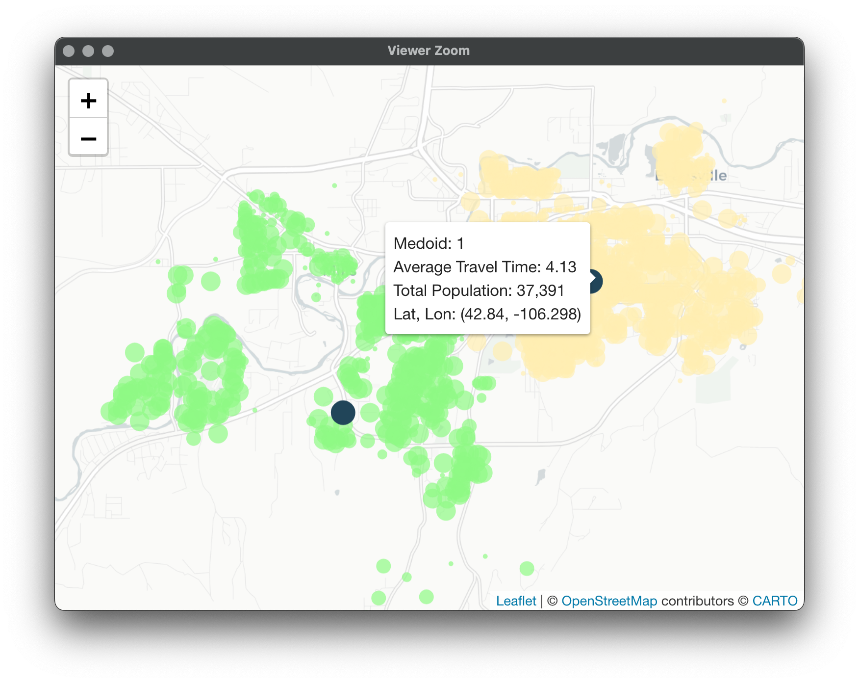
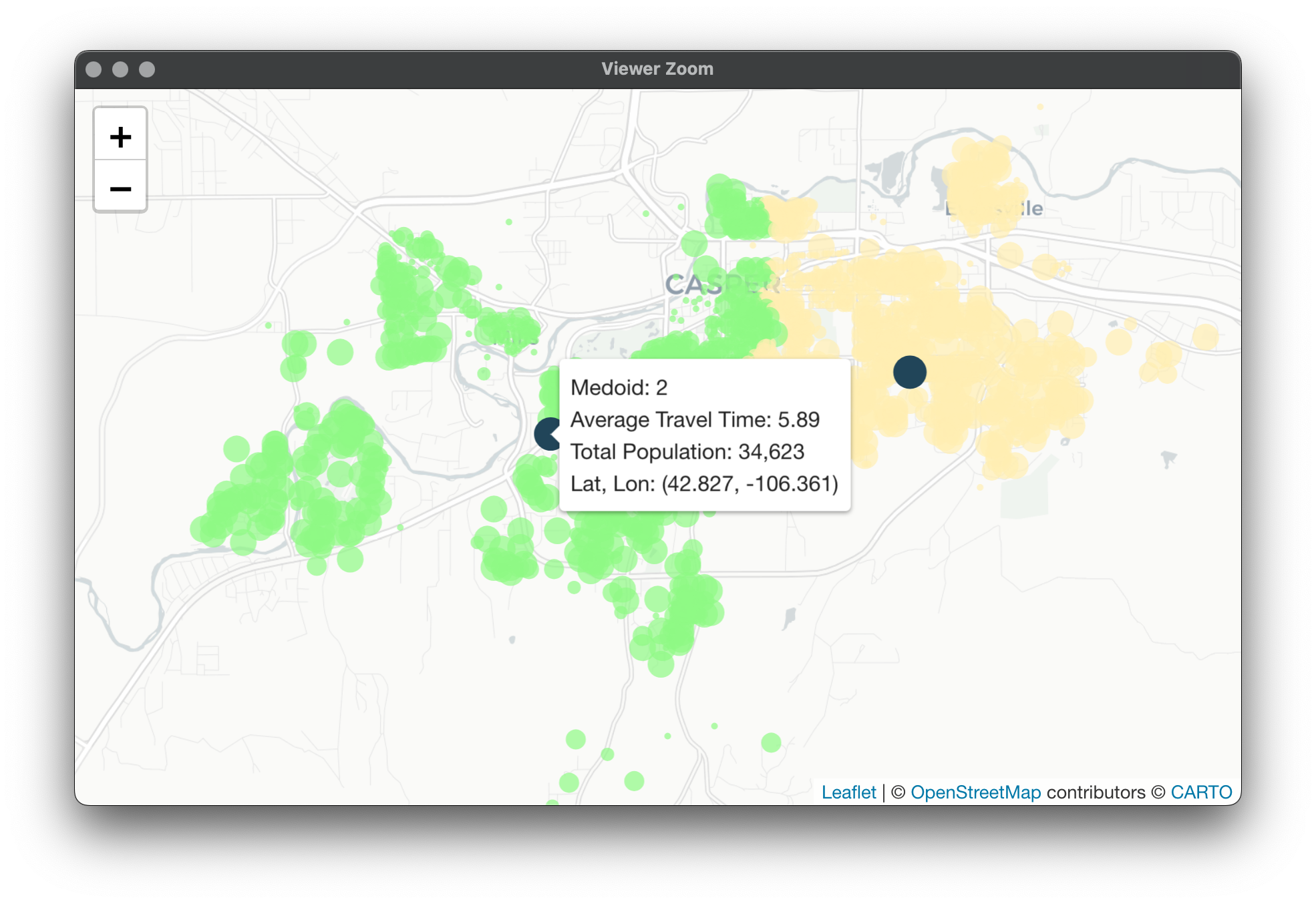
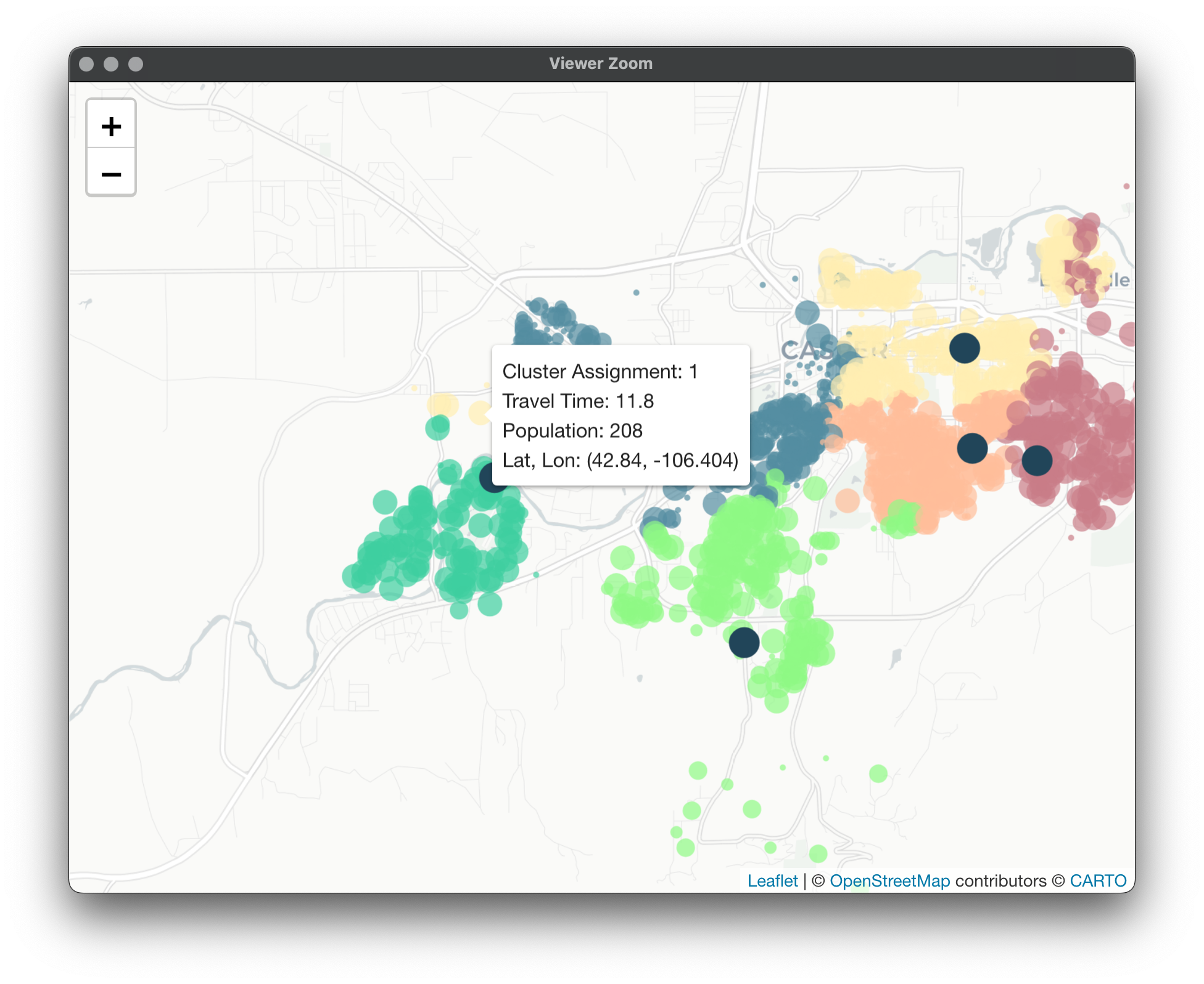
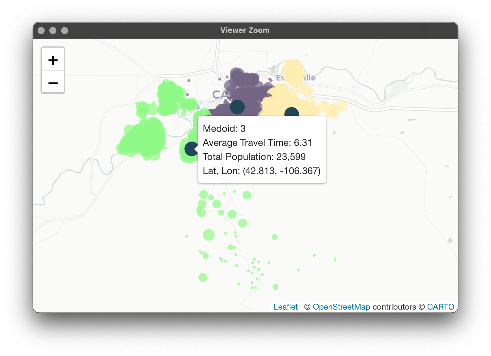
Here's the map for PAMonce with travel time: Here's for Equalify: What's interesting here is the minimal hit to average travel time despite the equalization of workloads. What about for 4 vans?
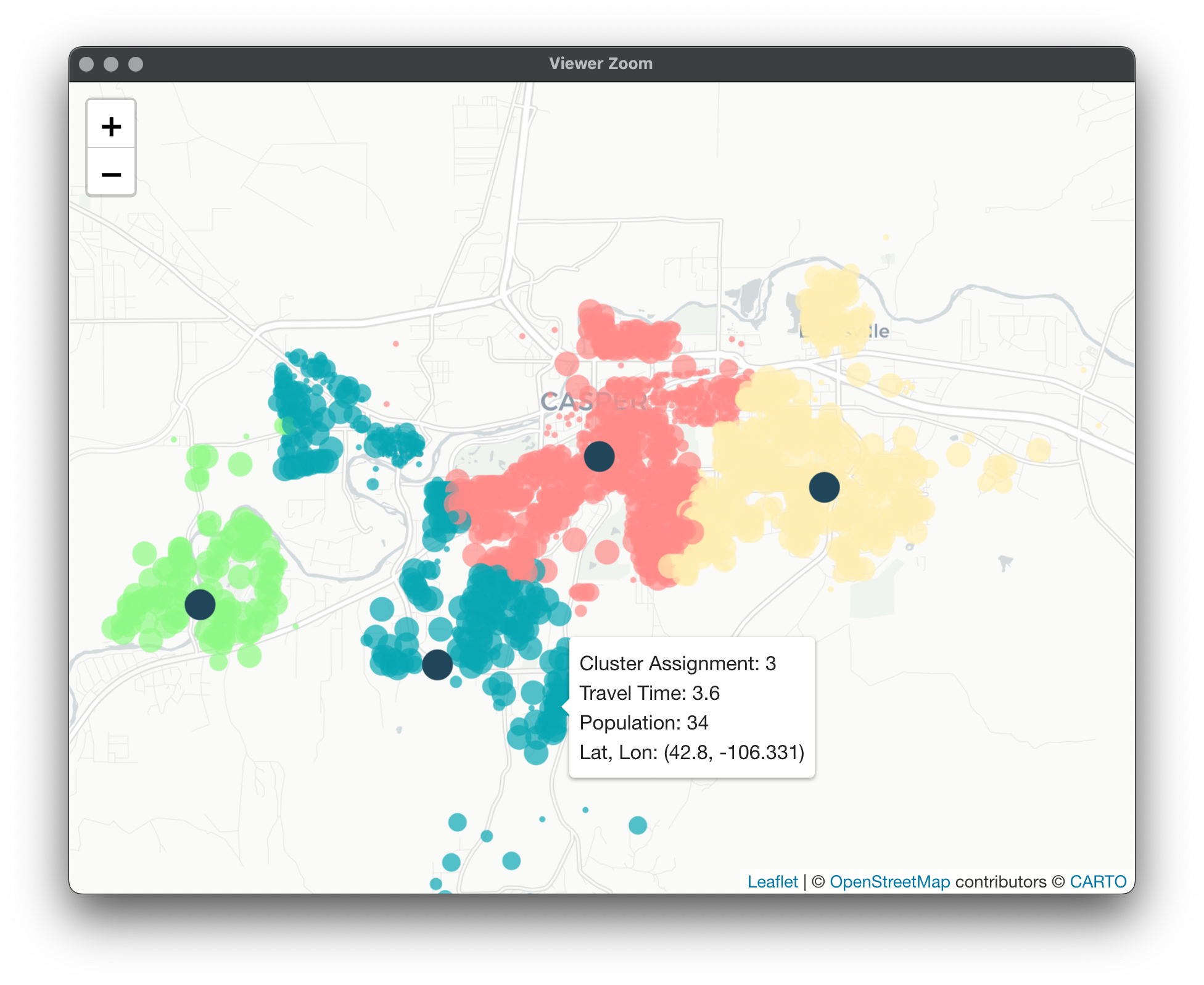
Map for PAMonce: Map for Equalify: These results are pretty interesting, while the cluster numbers are no longer directly comparable, there are a couple noticeable things. First would be that Equalify seems to be doing a decent job of sticking to its name with minimal losses to average travel time within each cluster. However, what we start to notice is a lack of nice separation between clusters 1 and 2 in this case.
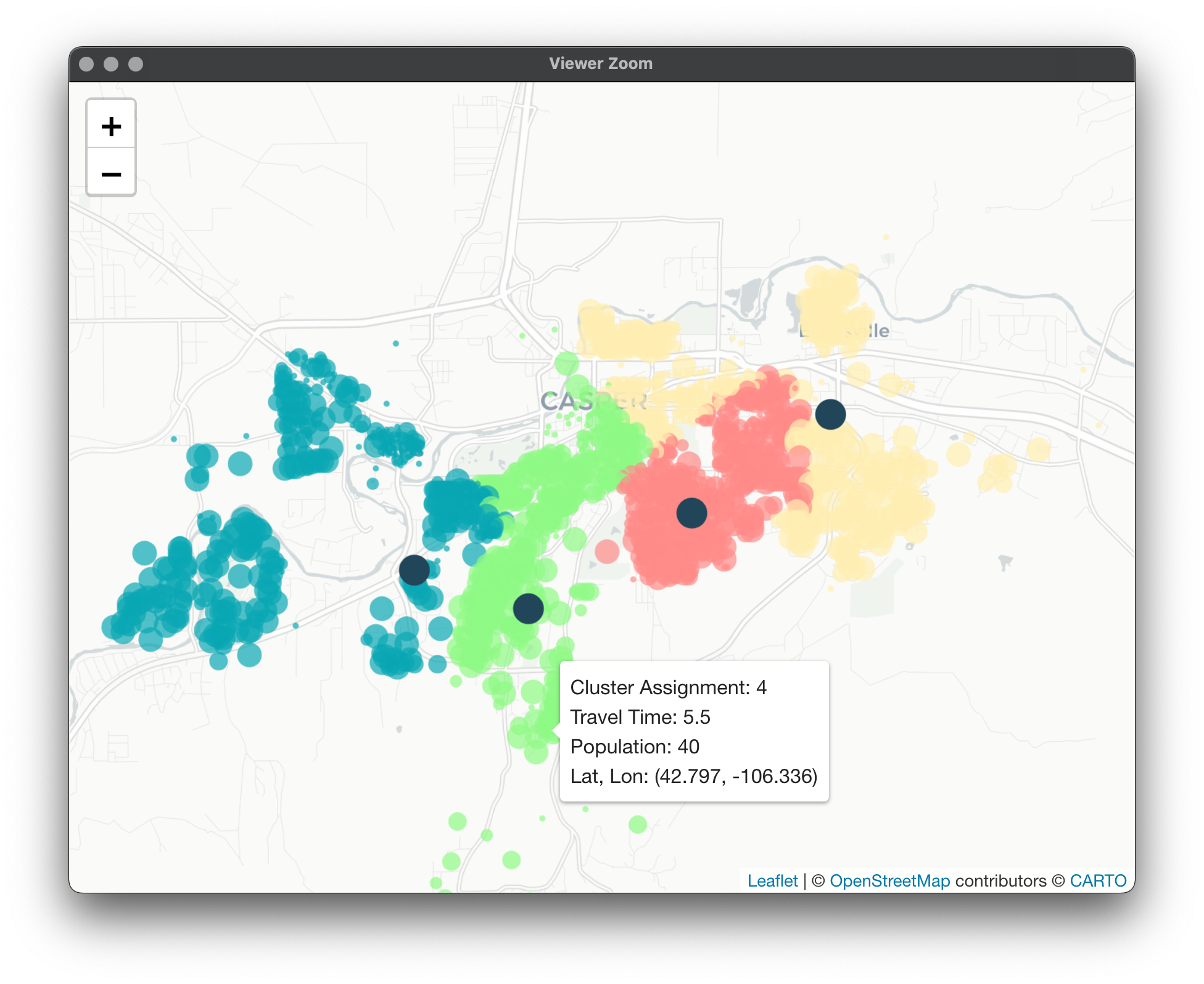
This is because our algorithm tries to account for travel times / spatial distances but isn't penalizing for lack of spatial distinctiveness. If we try 6 vans we can see more artifacts left behind because of the way we've set up Equalify.
Again here, it does a better job at equalizing workload but some odd artifacts are left behind. Take a look at these observations: Cluster 5 normally would've picked them up but its threshold criteria was met and so it missed out. Now they're assigned to a cluster halfway across town!
Discussion:
It's encouraging to see that Equalify seems to achieve its goal: equalizing workforce. As for the odd artifacts left behind, we could obviously manually assign the "leftovers" to clusters that make more sense. With minimal hits to travel time and vastly improved workloads between clusters, the clustering solutions offered by Equalify should still be considered despite their (sometime very obvious) shortcomings.
What might be of interest is adding some more reality into the mix here. We can do this by implementing discrete event simulation (DES). DES is interesting in this application, we can add things like vans "flexing" coverage. I.E., what happens when a van is currently being used and another delivery is requested? Should we wait for it to reset? Or, should another van that isn't being utilized "flex" over to take care of the new letter delivery? Some more items we can add are things like weather considerations depending on time of year. If you're familiar the Wyoming area, you know driving time can vary drastically in the winter time with icy-roads, etc.
Thus, the plan is to take our clustering solutions and put them head-to-head in a DES environment to see if any clear winners appear. Once the simulations are completed, we'll take the results and truly dig into them by building a shiny app as an investigative tool. This will no doubt be helpful to us when presenting our findings to the board!
